The Mann-Kendall trend test has become popular in the remote sensing community to test whether a time series of satellite observations is consistently increasing or decreasing. This consistency is referred to as monotonicity, and the function that describes it is called a monotonic function. On the other hand, a non-monotonic trend increases and decreases at different intervals in the time series.

A number of reasons are behind the popularity of the Mann-Kendall test in remote sensing: (1) it is a non-parametric test, which means it makes no assumptions on the distribution of the data. (2) It also does not assume the data to be homoscedastic, which means the variance around the regression line does not have to be the same for all values of the predictor variable. (3) It is resistant to outliers, so these do not have to be removed prior to trend detection.
The Mann-Kendall test does require that the data be independent and is sensitive to presence of serial correlation (i.e. data points are correlated with one another). This makes the null hypothesis of no trend to be rejected too frequently, making the test very liberal. In this case, it is might be useful to remove the serial correlation from the data through a process called prewhitening (case for prewhitening). On the other hand, if the sample size of the data and the magnitude of the trend are large, serial correlation does not affect the Mann-Kendall test statistics and prewhitening the data may remove part of the trend itself (case against prewhitening). So, the short answer on whether to prewhiten or not is that it depends on your data.
The Mann-Kendall test is usually performed on univariate time series such as hydrometeorological data derived from rain or streamflow gauges. However, satellite image time series has a different data structure that presents a unique challenge, i.e. each pixel is its own time series. While conducting analysis for the last research paper in my PhD, I developed a function in R that can take in raster stacks or bricks to perform the Mann-Kendall trend test and calculate its statistical significance (p values). The advantage of this function is that it only requires two R packages and only has two parameters, which makes it straightforward to run.
Tutorial: How to perform the M-K test on raster data in R
Here I’ve provided sample data to try out the function. The sample dataset comprises biweekly observations of normalized difference vegetation index (NDVI) over South America between 2000 and 2009. The spatial resolution is 0.5 degrees (~50km), so the dataset is not large (about 5.2 MB).
The function depends on the Kendall and raster packages in R, so you will need to install them. Once you’ve loaded them as well as custom function I’ve developed then you’re good to go.
require(raster)
require(Kendall)
# load NDVI time series stack from file.
ndvi.stack = stack("ndvi_SouthAmerica_2000-2009.tif")
# get the Mann-Kendall trend and p-values for the time series
system.time({mk.ndvi = MKraster(rasterstack = ndvi, type = "both")})
[1] "Start MKraster: 2020-10-18 13:03:42"
[1] "Loading parameters"
[1] "Done loading parameters"
[1] "Initiating loop operation"
[1] "Populating raster brick"
[1] "Ending MKraster on 2020-10-18 13:03:44"
user  system elapsed
2.06   0.00    2.06
As you can see, the trend analysis of the sample data took 2 seconds on my Windows 10/64-bit laptop with quad-core i7-8650U CPU, 32 GB RAM and running R 3.6.1 + R RStudio 1.2.1335. The duration will vary depending on your data and computing configuration. If you have a large dataset and a multicore computer, you can use the clusterR function from within the raster package to speed up the process.
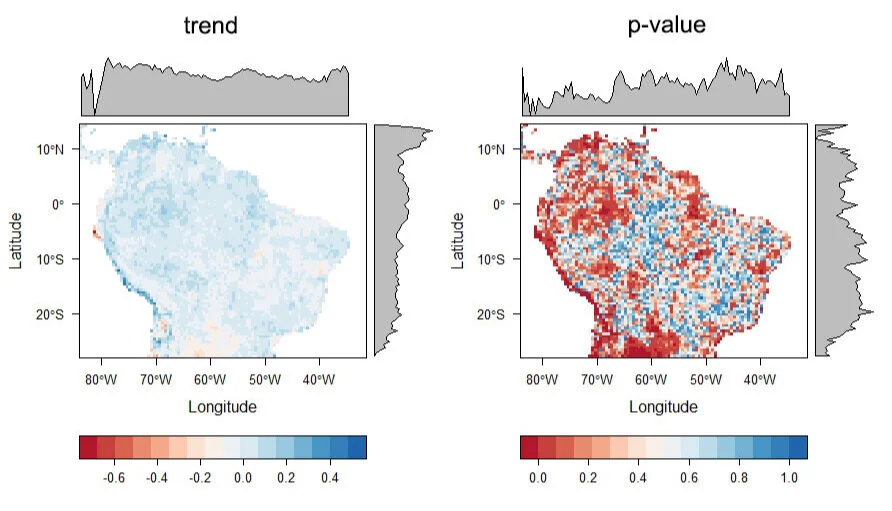
Using the sample NDVI data, this Mann-Kendall trend and its significance took 2 seconds on my laptop.